Pythonから利用できる数学処理ライブラリ、Scipyを使ったディジタルフィルタの設計・評価方法をまとめました。
と言っても数学的な話やディジタルフィルタについての概要は飛ばし、フィルタ設計・評価に使えるサンプルプログラムを載せただけですが、何かに使えれば幸いです。
サンプルコード
本記事で載せているコードの完全版は、以下パス先で共有しています
github.com
開発環境について
$wmic os get caption
>Microsoft Windows 10 Pro

$wmic os get osarchitecture
>64ビット

$python -V
Python 3.7.6

$pip list -V
scipy 1.4.1
目次
サンプルプログラム
代表的なIIRフィルタである以下フィルタの設計・評価のためのコードをまとめており、フィルタの周波数特性や位相特性、群遅延プロット、信号のフィルタ処理出力ができます。
※本記事ではまず移動平均フィルタのみを紹介
続きの記事
移動平均以外のフィルタ特性及びコードを載せています
dango-study.hatenablog.jp
- 移動平均フィルタ
- ButterWorseフィルタ
- 第一種Chebyshevフィルタ
- 第二種Chebyshevフィルタ
- Besselフィルタ
紹介するデジタルフィルタ出力例

※サンプリング 0.005sec
グラフ1つ目がフィルタの周波数特性
グラフ2つ目がフィルタの位相特性
評価用のサンプル信号について
フィルタ評価に使用するサンプル信号とサンプル信号の周波数特性を出力するコードです。
サイン波にノイズを足したものをサンプル信号とします。
dt = 0.005 #1stepの時間[sec]
fs = 1/dt
times  =  np.arange(0,10,dt)
N = times.shape[0]

f  = 5  #サイン波の周波数[Hz]
sigma  = 0.5 #ノイズの分散

np.random.seed(1)
# サイン波
x_s =np.sin(2 * np.pi * times * f)
x = x_s  +  sigma * np.random.randn(N)

x_np = np.array(x)

# サイン波+ノイズ
y_s =  np.zeros(times.shape[0])
y_s[:times.shape[0]//2] = 1
y = y_s  +  sigma * np.random.randn(N)

plt.figure(figsize=(12,6))
plt.subplot(3,1,1)
plt.plot(times, x, c="red", label=("sin+noise"))

#軸調整
plt.xlim(0,1)
plt.yticks([-2, -1.5, -1, -0.5, 0, 0.5,1, 1.5, 2])
plt.grid(which = "major", axis = "y", color = "gray", alpha = 0.8,
        linestyle = "--", linewidth = 1)
plt.legend()

def FFT(Raw_Data, sampling_time):
    sampling_time_f = 1/sampling_time
    fft_nseg = 256
    fft_overlap = fft_nseg // 2
    f_raw, t_raw, Sxx_raw = signal.stft(Raw_Data, sampling_time_f, nperseg=fft_nseg, noverlap=fft_overlap)

    return f_raw, t_raw, Sxx_raw

def get_start_end_index(t, start_t, end_t):
    start_ind=0
    while(t[start_ind] < start_t):
        start_ind += 1
    end_ind = start_ind + 1
    while (t[end_ind] < end_t):
        end_ind += 1
    return start_ind, end_ind

def ave_spectrum(Sxx, t, start_t, end_t):
    start_ind, end_ind = get_start_end_index(t, start_t, end_t)
    ave_spectrum = np.zeros(Sxx.shape[0])
    for i in range(Sxx.shape[0]):
        ave_spectrum[i] = np.average(Sxx[i, start_ind:end_ind])
    return ave_spectrum

f_raw, t_raw, Sxx_raw = FFT(x_np, dt)

plt.subplot(3,1,2)
plt.pcolormesh(t_raw, f_raw, np.abs(Sxx_raw),vmin=0, vmax=0.4, cmap="jet")

plt.subplot(3,1,3)
start = 0
end = 2
gain = ave_spectrum(np.abs(Sxx_raw), t_raw, start, end)
plt.plot(f_raw, gain, c="blue", label=("normal"))
plt.legend()

# プロット表示(設定の反映)
plt.show()
実行結果は以下の通りです。
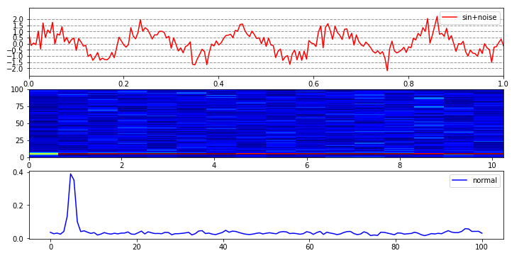
グラフ1つ目がサンプル信号の時系列です
グラフ2つ目がサンプル信号の周波数特性を示した時系列です。このグラフは関数「FFT」の出力結果で、横軸:時間 縦軸:周波数 色が出力(db)を示しており、周波数特性を時系列的に見たい場合に有効です。この画像だと5Hz付近で赤色となっており、グラフ3つ目の周波数特性とも合っていることが分かります。
グラフ3つ目がサンプル信号の周波数特性です。「start」「end」に時間を入力し、その時間範囲のデータでの周波数特性を示します。関数「FFT」の結果を関数「get_start_end_index」「ave_spectrum」で切り分け、平均化処理させた結果を描画しています。
移動平均フィルタについて
移動平均フィルタは、ローパスフィルタとして活用されます。
以下がサンプルコードとなり、フィルタ評価に使用するサンプル信号とサンプル信号の周波数特性を出力する関数です。
「move_num」移動平均個数であり、この値を変えていただくと、任意のフィルタについて評価できます。
「dt」サンプリングタイムであり、今回はサンプル信号に合わせています。
関数「character_MA」がフィルタ特性の出力用関数
関数「MA_filter」が実際のフィルタ処理用関数になります。
move_num = 5 #移動平均個数設定
dt = 0.005 #SamplingTime
fs = 1/dt  #周波数

class MA_Filter():
    def __init__(self, master=None):
        print("MA_Filter")

    def character_MA(self, N, fs, a=1):
        b = np.ones(N) / N
        fn = fs / 2# ナイキスト周波数計算

        w, h = signal.freqz(b, a)# 周波数応答計算
        x_freq_rspns = w / np.pi * fn
        y_freq_rspns = db(abs(h))#複素数をデシベル変換

        p = np.angle(h) * 180 / np.pi#位相特性
        w, gd = signal.group_delay([b, a])# 群遅延計算
        x_gd = w / np.pi * fn
        y_gd = gd

        return x_freq_rspns, y_freq_rspns, p, x_gd, y_gd

    def MA_filter(self, x, move_num):
        move_ave = []
        ring_buff = np.zeros(move_num)
        for i in range(len(x)):
            num = i % move_num
            if i < move_num:
                ring_buff[num] = x[i]
                move_ave.append(0)
            else:
                ring_buff[num] = x[i]
                ave = np.mean(ring_buff)
                move_ave.append(ave)
        return move_ave

MFilter = MA_Filter()
フィルタ特性について
フィルタ特性確認用のサンプルコードです。
x_freq_rspns_ave, y_freq_rspns_ave, p_ave, x_gd_ave, y_gd_ave = MFilter.character_MA(move_num, fs, a=1)

# グラフ表示
plt.figure(figsize=(12,6))
# 周波数特性
plt.subplot(3, 1, 1)
plt.plot(x_freq_rspns_ave, y_freq_rspns_ave)
plt.xlim(0, 100)
plt.ylim(-200, 2)
plt.ylabel('Amplitude [dB]')
plt.grid()

# 位相特性
plt.subplot(3, 1, 2)
plt.plot(x_freq_rspns_ave, p_ave)
plt.xlim(0, 100)
plt.ylim(-200, 200)
plt.xlabel('Frequency [Hz]')
plt.ylabel('Phase [deg]')
plt.grid()

# 群遅延プロット
plt.subplot(3, 1, 3)
plt.plot(x_gd_ave, y_gd_ave)
plt.xlim(0, 100)
plt.ylim(-5, 15)
plt.xlabel('Frequency [Hz]')
plt.ylabel('Group delay [samples]')
plt.grid()
plt.show()
実行結果は以下の通りです。

グラフ1つ目がフィルタの周波数特性
グラフ2つ目がフィルタの位相特性
グラフ3つ目がフィルタの群遅延を示しています。
群遅延は、フィルタ処理によって何サンプル分信号が遅れるのかを示しており、その確認ができます。
フィルタ処理結果の確認
フィルタ処理結果確認用のサンプルコードです。
「x」に任意の信号を入れていただくことで処理ができますので、処理したい信号を「x」に入れて試してみてください。
moveave_x = MFilter.MA_filter(x, move_num)

plt.figure(figsize=(12,6))
plt.subplot(3,1,1)
plt.plot(times, x, c="red", label=("sin+noise"))
plt.plot(times, x_s, c="blue", label=("sin"))
plt.plot(times, moveave_x, c="green", label=("MA"))

#軸調整
plt.xlim(0,1)
plt.yticks([-2, -1.5, -1, -0.5, 0, 0.5,1, 1.5, 2])
plt.grid(which = "major", axis = "y", color = "gray", alpha = 0.8,
        linestyle = "--", linewidth = 1)
plt.legend()

f_raw, t_raw, Sxx_raw = FFT(x_np, dt)
plt.subplot(3,1,2)
plt.pcolormesh(t_raw, f_raw, np.abs(Sxx_raw),vmin=0, vmax=0.4, cmap="jet")

plt.subplot(3,1,3)
start = 0
end = 2
f_raw, t_raw, Sxx_raw = FFT(x, dt)
gain = ave_spectrum(np.abs(Sxx_raw), t_raw, start, end)
plt.plot(f_raw, gain, c="red", label=("sin+noise"))
f_raw, t_raw, Sxx_raw = FFT(x_s, dt)
gain = ave_spectrum(np.abs(Sxx_raw), t_raw, start, end)
plt.plot(f_raw, gain, c="blue", label=("sin"))
f_raw, t_raw, Sxx_raw = FFT(moveave_x, dt)
gain = ave_spectrum(np.abs(Sxx_raw), t_raw, start, end)
plt.plot(f_raw, gain, c="green", label=("MA"))
plt.legend()

# プロット表示(設定の反映)
plt.show()
実行結果は以下の通りです。

グラフ1つ目の緑プロットが移動平均フィルタ後の出力となります。※フィルタ処理前が赤プロット
グラフ2つ目がフィルタ後出力の周波数特性を示した時系列です。
グラフ3つ目の緑プロットが移動平均フィルタ後の周波数特性になります。
今回作成した移動平均フィルタのフィルタ特性を見ると、20Hz付近から減衰するようなフィルタ特性を持っており、グラフ3つ目の緑プロットと赤プロットを比較して、設計通りのフィルタが作成できていることが分かります。
まとめ
今回はScipyを使ったディジタルフィルタの設計・評価で使えるコードを紹介しました。
フィルタ特性を確認と評価が合わせてできるように作成したので、使えるケースもあるかもしれません。
IIRの別のフィルタについても書いていく予定です。